I am reading the research paper titled Introduction to convolutional neural networks by Keiron O’Shea and Ryan Nash.
Here is what I learned after reading the paper.
Before learning convolutional neural networks, it is important to understand the neural networks and their limitations.
Artificial Neural Networks
What are neural networks?
The neural networks are inspired by the human biological system, highly influenced by neurons in the brain.
Architecture of Neural Networks

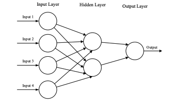
Fig: Layered Neural Network
- The input loaded as vector form
- The circles in the above figure called nodes.
- The output of each layer is sent to next layer as input, These layers are called hidden layers.
- The last layer is called the output layer.
- The number of nodes in the output varies based on the specific type of problem.
The mathematical notation of node.
Let’s say the input to the node is x1. The output of the node can be written as:
\[output = f(x_1 \cdot w_1 + w_0)\]W1 and W0 are called weights. In order to adjust the weights, optimization algorithms such as gradient descent, adam and newton methods etc. are used to get the desired output.
The term f is called activation function. Head over to activation to read more.
Limitations of Neural Networks
Artificial neural networks tend to struggle with image data. Let’s take the image of dimension 28x28. The number of weights in single neuron would be 784. If the input image is colored and of dimensions 61x61x3. The total number of weights in just one neuron is 12288. As the image input scales, the increase in the number of weights is substantial. Convolutional neural networks are best suited to deal with large image dimensions.
Convolutional Neural Network
What are convolutional neural networks?
Ans:Convolutional Neural Networks are type of neural networks used to improve the performance of traditional neural networks while processing the image, video or audio data.

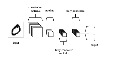
Credits: Paper,Simple CNN Architecture Consists of 5 Layers
Convolutional neural networks usually consist of 3 types of layers
- Convolutional Layer
- Pooling Layer
- Fully-Connected Layer
Let’s understand each layer in detail.
Convolutional Layer
This is the crucial part in the convolutional neural networks. In Convolutional layer the input is convolved with kernels, and we get the output.
The output dimension of each layer is calculated as follows:
\[(W − F + 2P) / S) + 1\]W is the width/height of input image and F is the width/height of the kernel, kernels are represented by the weight matrix and P is a padding and S is a stride.
Padding: The amount of pixels added around the original image.
Strides: Step size used when sliding the filters .

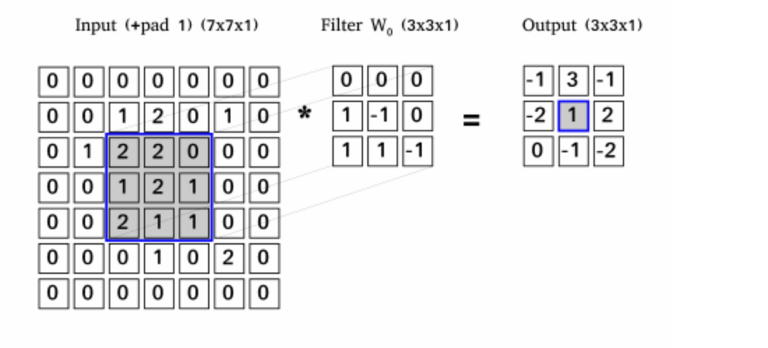
Credits: www.cosmos.esa.int
The above image is 6x6 with a padding 1 and kernel size is 3x3. The output value of the middle pixel can be calculated as 2(0)+2(0)+0(0)+1(1)+2(-1)+1(0)+2(1)+1(1)+1(-1) = 1
Pooling Layer
The pooling layer reduces the number of parameters and computational complexity of the model. Most CNNs use max pooling, with a kernel size of 2x2 and strides of 2. It scales down the original image by 25% while maintaining its depth.
Fully Connected Layer
The last layers are fully connected neural networks. It is same as the artificial neural networks with the property of every node in one layer connected with the one node of previous layer.
Sample code to create the CNN using Keras
import tensorflow as tf
from keras.models import Sequential
from keras.layers import Conv2D, MaxPooling2D, Flatten, Dense
# Create the CNN model
model = Sequential()
The Sequential model allows us to create a neural network by adding layers sequentially, one after the other. Let’s go ahead and add convolutional, padding and fully connected/dense layers.
# Convolutional layer with 32 filters, a 3x3 kernel, and ReLU activation
model.add(Conv2D(32, kernel_size=(3, 3), activation='relu', input_shape=(28, 28, 1)))

# Max pooling layer with 2x2 pool size
model.add(MaxPooling2D(pool_size=(2, 2)))

# Convolutional layer with 64 filters and a 3x3 kernel
model.add(Conv2D(64, kernel_size=(3, 3), activation='relu'))

# Max pooling layer
model.add(MaxPooling2D(pool_size=(2, 2)))

# Flatten the output
model.add(Flatten())

# Fully Connected layer
model.add(Dense(128, activation='relu'))

# Output layer with 10 neurons (for 10 classes) and softmax activation
model.add(Dense(10, activation='softmax'))
# Print a summary of the model
model.summary()
The output of the above snippet is.
Model: "sequential"
_________________________________________________________________
 Layer (type)                Output Shape              Param #
=================================================================

 conv2d (Conv2D)             (None, 26, 26, 32)        320

 max_pooling2d (MaxPooling2D)  (None, 13, 13, 32)       0

 conv2d_1 (Conv2D)           (None, 11, 11, 64)        18496

 max_pooling2d_1 (MaxPooling  (None, 5, 5, 64)         0
 2D)

 flatten (Flatten)           (None, 1600)              0

 dense (Dense)               (None, 128)               204928

 dense_1 (Dense)             (None, 10)                1290

=================================================================
Total params: 225,034
Trainable params: 225,034
Non-trainable params: 0
_________________________________________________________________
I have a CIFAR_CNN.ipynb notebook in my GitHub which is a machine learning model implementation using Convolutional Neural Networks (CNNs) for the CIFAR-10 dataset. This notebook showcases how to build a CNN model to classify images from the CIFAR-10 dataset, which consists of 60,000 32x32 color images belonging to 10 different classes. Feel free to fork the notebook.
https://github.com/gopikrsmscs/MachineLearningModels/blob/main/CIFAR_CNN.ipynb
Thank you for taking your time to read my blog post. I hope you found it informative and enjoyable. I would love to hear your thoughts and engage in a discussion section.
If you like what you read feel free to like, share and follow in LinkedIn.